


Inventory practice: Quality assurance (QA) and quality control (QC) in Norway‘s GHG inventory

Keywords: QA/QC

Norway’s inventory uses a range of methods to ensure quality assurance (QA) and quality control (QC). These include:

Check that assumptions and criteria for the selection of activity data and emissions factors are documented: Thorough checks of emission factors and activity data and their documentation are performed for all emission sources.

Check for transcription errors in data input and references: Activity data are often statistical data. Official statistical data undergo a systematic revision process, which may be manual or, increasingly frequently, computerized. The revision significantly reduces the number of errors in the statistics used as input to the inventory. All input data (reported emissions, emission factors and activity data) for the latest inventory year are routinely compared to those of the previous inventory year, using automated procedures. Large changes are automatically flagged for further, manual QC.

Check that emissions are calculated correctly: When possible, estimates based on different methodologies are compared.

Check that parameter and emission units are correctly recorded and that appropriate conversion factors are used: All parameter values are compared with values used in previous years and with any preliminary figures available. Whenever large deviations are detected, the value of the parameter in question is first checked for typing errors or unit errors. If necessary, the primary data suppliers are contacted for explanations and possible corrections.

Check the integrity of database files: Control checks of whether appropriate data processing steps and data relationships are correctly represented are made for each step of the process. It is verified that data fields are properly labelled, have correct design specifications and that adequate documentation of database and model structure and operation are archived.

Check for consistency in data between source categories: Activity data and other parameters that are common to several source categories should be evaluated for consistency, e.g. activity data used for enteric fermentation, methane and nitrous oxide manure management emissions.

Check that the movement for inventory data among processing steps is correct: Statistics Norway has established automated procedures to check that inventory data fed into the model does not deviate too much from the estimates for earlier years, and that the calculations within the model are correctly made. Checks are also made that emissions data are correctly transcribed between different intermediate products. The model is constructed so that it gives error messages if factors are lacking, which makes it quite robust to miscalculations.

Undertake review of internal documentation: For some sources, expert judgements dating some years back are used with regard to activity data/emission factors. In most of the cases these judgements have not been reviewed since then, and may not be properly documented, which may be a weakness of the inventory. The procedures have improved the last few years, and the requirements for internal documentation to support estimates are now quite strict; all expert judgements and assumptions made by the Statistics Norway staff should be documented.

Check of changes due to recalculations: Emission time series are recalculated every year to ensure time series consistency. The recalculated emission data for a year are compared with the corresponding estimates from the year before.

Undertake completeness checks: Estimates are reported for all source categories and for all years to the best of our knowledge. During the implementation of the 2006 IPCC Guidelines, a systematic evaluation of all potential new sources was performed.

Compare estimates to previous estimates: Internal checks of time series for all emission sources are performed every year when an emission calculation for a new year is implemented. It is examined whether any detected inconsistencies are due to data and/or methodology changes.


Author: Andreas Wilkes, Values for development Ltd (2019)
Inventory practice: Quality assurance (QA) and quality control (QC) in Poland’s GHG inventory

Keywords: QA/QC | institutional arrangements

Poland’s inventory compilation agency, National Centre for Emission Balancing and Management (KOBiZE), has put in place a quality assurance (QA), quality control (QC) and verification program for the annual GHG inventory.

QC activities are carried out by the personnel directly responsible for the inventory and are aimed at maintaining standards and quality. The main QA activities conducted are Tier 1 methods applied to all sources and sinks. Tier 2 procedures are applied to key categories (including enteric fermentation). QC covers routine technical activities to maintain the correctness and completeness of data and eliminate errors and determine potential deficiencies. Checks are made on the accuracy of data and the procedures for calculation of emissions, uncertainty, archiving of information and reporting.

QA covers procedural systems for control carried out by experts not involved directly in compiling the inventory in a given sector. QA activities are conducted on a completed inventory and aim to ensure that national inventory represents the best level of knowledge and available data, and to support QC.

Verification activities include comparisons with external emission analyses estimates and databases prepared by independent bodies or teams. They allow to improve inventory methods and outcomes in both the short and long term.

The KOBiZE Data Management Manual describes the inventory requirements for databases, software, worksheets, final reports as well as QA/QC documentation. Documentation of data and calculation QC are archived in electronic and hardcopy forms. The main procedures for QA/QC activities are described in the National Quality Assurance Quality Control and Verification Program of the Polish Greenhouse Gas Inventory and the detailed QC procedures are procedures performed by KOBiZE experts.

Table 1 summarizes the timeframe for inventory compilation and QA/QC activities. The dates for particular stages are established based on country specific availability of statistical data as well as national (legal) and international obligations.

Table 1: Timetables for inventory preparation and check (n-submission year) in Poland

TimingActivity
June 15 December (year n-1)• Data and emission factor collection (estimation)
• Check for consistency and correctness of emission data, trends and factors, using QC and verification methods
• Initial calculations and checks of GHG emissions
• Submission to Ministry of Environment for acceptance
15 January (year n-2)• Submission of GHG inventory for the year n-2 and elements of NIR to EIONET CDR as required by EU regulations
15 December 15 February (year n-2)• Emission results and methodology verification based on comments from ministerial emission experts (QA methods applied)
• Elaborate final inventory, additional checks and final corrections, preparation of NIR and CRF tables (QC and verification methods applied)
• Submission to Ministry of Environment for acceptance
15 March (year n-2)• Emission results and methodology verification based on comments by external sector experts in inter-ministerial check of the report (QA methods applied)
• Submission of NIR and CRF tables to EIONET CDR as required by EU regulations
15 April (year n-2)• Submission of GHG inventory for the year n-2 to UNFCCC secretariat (NIR and CRF tables)

Source: Poland NIR 2017

Each inventory sector undergoes detailed QC procedures carried out by a designated expert during its preparation, after completing the calculations, after generating the CRF tables generation and after completing the NIR report.

As a part of QA activity, the inventory team cooperates with specialists from different institutes, associations and individual experts who are involved in verification of data and assumptions to the inventory. Domestically, once the NIR is delivered to the Ministry of Environment, it undergoes internal consultation among departments, and external consultation through inter-ministerial dialogue, during which agencies sub-ordinate to the relevant ministry review the inventory. QA is also performed by EU and UNFCCC agencies.

After including obtained comments and amendments into the NIR, the NIR is sent to the European Commission where inventory results and methodology are also discussed. The national inventory results are also verified by the European Union. Since 2012 this verification is performed using the EEA Emission Review Tool (EMRT, EEA Review Tool).

The results of the submitted CRF files are also controlled by the UNFCCC Secretariat, and annual international review of the Polish GHG inventory under UNFCCC is a key element in the process of quality improvement.


Author: Andreas Wilkes, Values for development Ltd (2019)
Inventory practice: Structured elicitation of expert judgement on manure management systems in Canada

Keywords: Manure management | Surveys | Expert judgement

What data needs were addressed? Information on manure management practices.

Why was the data needed? In Canada’s initial inventories in the 1990s, the distribution of manure management practices was estimated using expert judgement by a small number of experts. Some government data was available, but only for a small number of manure management systems and a few livestock types. Improved estimates reflecting the diversity of practices across the country were needed.

Methods used: Surveys of regional experts.

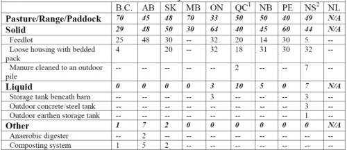
How was the data need addressed? Before designing the survey was designed, it was necessary to define the major manure management practices in the country so that the survey is in line with IPCC definitions of manure management systems as well as reflecting national conditions. This was done by the contracted researcher in collaboration with two manure experts. The survey was then designed and sent to 68 experts in different provinces, including government staff as well as private sector waste management experts. Responses were received from 16 experts. The survey tool asked each person to read the definitions of manure management systems and to indicate the percentage of manure in each system for each type of livestock in their province. Where more than one response was received from the same province, the average value was taken. The survey results were then compared to the existing limited government data, which confirmed the dominant patterns of manure storage methods reflected in the government survey. Table 1 shows the summary results for beef cattle in different provinces.

Table 1: Percent distribution of manure management practices by province for beef cattle

Source: Marinier et al. 2004

Since production systems have not changed significantly, Canada’s inventory continues to use this distribution of manure management practices, combined with annual data on the population of livestock in each province, which changes from year to year. However, academic studies have pointed to some ways in which Canada’s manure management emission estimates could be improved (Vanderzaag et al. 2013).


Further Resources

Marinier M, et al. 2004. Determining manure management practices for major domestic animals in Canada. Environment Canada, unpublished report.

VanderZaag AC, et al. 2013. Towards an inventory of methane emissions from manure management that is responsive to changes on Canadian farms. Environmental Research Letters.


Author: Andreas Wilkes, Values for development Ltd (2019)
Inventory practice: Estimating number of days alive

Keywords: Livestock population | surveys | interpolation | expert judgement

IPCC Guidance suggests that the livestock population data used should be the annual average population:

Annual average population = days_alive * (number of animals produced annually 365)

Many countries do not report in detail how the number of days alive is estimated for cattle, focusing mainly on the gradual growth of cattle populations over time. For beef finishing cattle, swine and poultry, however, estimation of days alive is more common. Countries use various methods to estimate the annual average population and number of days alive. Some examples include:

Modeling different production stages using expert judgement: Canada’s inventory uses cattle subcategory population data from national statistics (e.g. cows, heifers, steers etc). Each sub-category is then divided into production stages (e.g. background heifers and steers, finishing heifers and steers, short- and long-finish feedlot heifers and steers). The proportion of each subcategory backgrounded or on feedlot, and the duration on feedlots until marketing were estimated using expert judgement elicited through a nationwide survey of livestock experts (see Inventory Practice: Structured elicitation of expert judgement in Canada’s initial Tier 2 inventory). The inventory estimates GE and CH4 emissions per subcategory of animal, considering also the number of days spent in each production stage.

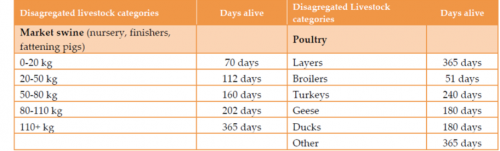
Expert judgement: Croatia’s Tier 2 inventory uses expert judgement from the Faculty of Agriculture at the University of Zagreb estimate the number of days alive for swine and poultry:

Table 1. Livestock categories and days alive estimated to calculate annual average population in Croatia

Source: Croatia NIR 2017

Similarly, South Africa’s inventory uses research that assumed feedlot cattle are kept on the feedlot for 110 days (i.e. assuming 3 cycles per year).

Many countries also adjust emission factors for calves before weaning and consider that enteric fermentation emissions are significant only after weaning. The duration of suckling is mostly determined by expert judgement.


Further Resources

Du Toit CJL, Van Niekerk WA. 2013. Direct methane and nitrous oxide emissions of South African dairy and beef cattle. South African Journal of Animal Science.


Author: Andreas Wilkes, Values for development Ltd (2019)
Livestock inventory practice: Characterization of manure management systems in Finland

Keywords: Manure management | surveys | interpolation | cattle | Europe

What data needs were addressed? To quantify the allocation of manure among different manure management systems.

Why was the data needed? The Finnish government does not collect data on manure management systems in a format suitable for use in the inventory. Prior to 2014, Finland’s inventory used expert judgement applied to limited data from a government survey to characterize the allocation of manure to different management systems. An improved estimate was needed.

Methods used: farm survey, interpolation

How was the data need addressed? As part of a study funded by the environment agency to identify ways to reduce ammonia emissions, a new questionnaire was made and sent to more than 11,000 farms, of which approximately 23% replied. Based on the data collected, activity data on the shares of manure management systems for 1990 to 2005 were kept the same as before (except for dairy) but from 2006 onwards the values were updated. The 2012 management system data was updated and data for years between 2006 and 2011 were interpolated. The values from 2013 onwards are based on an estimated trend between 2012 and 2020 that assumes the share of slurry will continue to increase.

It is planned in the future to improve data on the share of manure in dry lots, which are currently estimated at about 1-3% of excreted manure.


Further Resources

Grönroos J. 2014. Reduction possibilities and costs of agricultural ammonia emissions. (Written in Finnish)


Author: Andreas Wilkes, Values for development Ltd (2019)

Inventory practice: Livestock population estimates in Croatia

Keywords: Livestock population | extrapolation | expert judgement

What data needs were addressed? To construct a time series for livestock populations.

Why was the data needed? Croatia has used a Tier 2 approach for cattle emissions since 2009. Cattle are categorized as mature dairy cows, mature non-dairy animals and calves. The challenges were to reconstruct time series for each of the cattle sub-categories when national official statistics were not available for all years, and the sub-categorizations in national statistics changed over time.

Methods used: extrapolation, expert judgement.

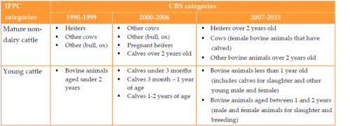
How was the data need addressed? The Croatian Bureau of Statistics (CBS) holds data on other cattle since 1990. Numbers of dairy cattle were provided by the Croatian Agricultural Agency (CAA) for the years 2008-2015. For 1990 to 2007, dairy cattle numbers were extrapolated based on the 2008-2015 numbers using expert opinion from the Croatian Agency for the Environment and Nature. For non-dairy cattle, the sub-categories reported by the CBS has changed over time. The table below shows how different categories were mapped onto the IPCC categories over time.

Table 1: Changing classifications of non-dairy cattle in Croatia


Author: Andreas Wilkes, Values for development Ltd (2019)

Inventory practice: Estimating livestock population time series in Romania

Keywords: Livestock population | extrapolation | expert judgement

What data needs were addressed? To construct a time series for livestock populations.

Why was the data needed? Prior to 2012, Romania used a Tier 1 approach for all livestock types. National primary data on the total number of cattle was sufficient for a Tier 1 approach. When a Tier 2 approach was adopted, a time series for the population of cattle sub-categories was needed, but official data did not report cattle sub-categories until 2004.

Methods used: extrapolation, expert judgement, comparison with FAO and EUROSTAT databases.

How was the data need to be addressed? An institute was contracted to produce a time series for the population of cattle sub-categories. Based on their proportions in the 2004 data, for 1989-2003, the following proportions of sub-categories in the total cattle population were assumed:

  • Dairy cattle are 56% of the total cattle population
    Among non-dairy cattle,
  • calves for slaughter < 1 year old represent 10.03% of total cattle;
  • young cattle for breeding < 1 year old represent 15.3% of total cattle;
  • young cattle for breeding between 1-2 years represent 7.97% of total cattle
  • male cattle >2 years 0.34%
  • female cattle >2 years 5.83%
  • males and females > 2 years for slaughter 1%
  • cattle for work 1.94%.

Assuming a constant herd structure was in line with expert opinion that herd structure did not change significantly over this period. Since 2004, primary data on all sub-categories have been collected by the National Institute of Statistics (NIS). The data are published in the Statistical Yearbook of Romania and reported by NIS to EUROSTAT, which also publishes the data.

In 2015, the primary livestock population time series were verified by comparing the data in the inventory with data published by FAO and EUROSTAT. It was found that EUROSTAT data round livestock populations to the nearest hundred, causing small errors in the time series. Differences with FAO data were due to the fact that the values for the year X are allocated by FAO of year X-1, and to rounding.


Author: Andreas Wilkes, Values for development Ltd (2019)

Inventory practice: Structured elicitation of expert judgement in Canada’s initial Tier 2 inventory

Keywords: Expert judgement | surveys| milk yield | animal weight | weight gain

What data needs were addressed? Information on management practices and performance of cattle.

Why was the data needed? When Canada first adopted a Tier 2 approach, various sources of information on cattle production practices and performance were used. Initially, data from surveys published in scientific journals was used, but this was not available for all animal sub-types.

Methods used: Surveys of regional experts.

How was the data need addressed? Surveys posing questions on dairy and beef production practices were administered to about 100 cattle specialists at the regional and/or provincial level in the country, with fewer (e.g. 6) specialists contacted in provinces with smaller cattle populations and more (e.g. 15) contacted in provinces with larger populations. The survey asked the specialists to provide estimates for key parameters (e.g. average weight, mature weight, weight gain and weight loss during lactation, milk yields, conception rates) and to describe key production practices (e.g. time spent in confinement and on pasture in a year, type of feed fed (type of grain and hay/silage fed) and % of grain in the diet).

The data from the surveys were then collated in a table together with existing published data and other data sources (e.g. personal communications from experts on particular topics). Examples selected from the collated results of the survey are given in Table 1. In this way, the survey data were used to fill data gaps in the inventory. For example:

  • Milk yield and milk fat data: records of milk yield were available for 8 provinces. For 2 provinces with no recorded data, survey data were used.
  • Animal weight and weight loss: Survey data on weight loss were used for 2 provinces where no other data source was available.
  • Production practices (e.g. housing, grazing, feed) were estimated based on the predominant practice in each province.

Table 1: Collation of structured survey data and literature values for dairy cows in one Canadian province (values with no given source are from the survey)

Dairy cows
Average weight (kg)700
Mature weight (kg)700
Daily weight gain (kg/d)0.7 (young stock), 0.3 (cows)
Weight loss (kg/d)-1.28 for first 70 days of lactation
Milk (kg/d)33.0
31.9 (recorded data)
Milk fat (%)3.5
3.6 (recorded data)
Conception rate (%)55 (first service)
67 (Usenik, pers. comm.. with first service based on only 30% of population)
Days in milk (d)351 (survey estimate)
351 (recorded)
Days dry (d)75 (survey estimate)
75 (recorded)
Production environment95% confinement housing, dry cows in dry pens for 7-8 weeks, and 1 week in calving pen
FeedTMR (60% forage, 40% concentrate) for 351 days

The survey results were compiled in an internal report, a summary of which was published in Ominksi et al (2007), and results were incorporated into Canada’s national inventory (2005).


Further Resources

Bondi D, et al. 2004. Improving Estimates of Methane Emissions Associated with Enteric Fermentation of Cattle in Canada by Adopting an IPCC (Intergovernmental Panel on Climate Change) Tier-2 Methodology. Unpublished report.

Ominski KH, et al. 2007. Estimates of enteric methane emissions from cattle in Canada using the IPCC Tier-2 methodology. Canadian journal of animal science.


Author: Andreas Wilkes, Values for development Ltd (2019)

Inventory practice: Regional characterization of dairy cattle in New Zealand

Keywords: Livestock characterization | dairy cattle

What data needs were addressed? Regional characterization of dairy cattle.

Why was the data needed? New Zealand’s initial Tier 2 approach allocated the livestock population to 3 different types of grassland (i.e. improved, unimproved and tussock) in 4 climate zones. Later analysis suggested that allocating all animals to 1 climate region and 1 of grassland changed total methane emissions by around 1% (Clark, 2001). So when a revised Tier 2 approach was adopted in 2002, detailed spatial categorization was no longer used. To account for differences in dry matter intake and methane conversion rates (Ym), weighted averages based on the proportion of animals in each pasture type were used. However, by the second half of the 2000s, the dairy sector had undergone rapid change, with large increases in the dairy population and productivity in some regions. This meant that a single national model for dairy emissions may no longer be accurate.

Methods used: Regional characterization of dairy cattle.

How was the data need addressed? A study (Clark, 2008) was undertaken to compare the differences in dairy cattle emissions estimated using a single national model and an aggregation of regional models. The study identified data on dairy cattle populations and animal performance that were both available at the regional level. Official population data were available for 73 Local Territory Authorities, while the animal performance data (i.e. total milk produced, milk fat and protein content, weight of dairy cows by breed and proportion of each breed in the national herd) were available from a farmer cooperative disaggregated into 17 regions. Both data sources provided time series going back to 1990. These data sources were already used in the national inventory. Therefore, the comparison was a test of whether the national GHG emissions model was linear or not; if it was linear, national and aggregated regional estimates would be identical.

The results showed that for 1990, the two models yielded very similar results. However, for 2006, differences were more significant, with the regional model estimating 2.3% lower national dairy cattle emissions than the national model. The trend in emissions is therefore non-linear. The reason is that emissions are most directly related to feed consumption, but feed consumption is estimated on the basis of animal performance (e.g. milk yield, live weight), which is not linearly related to feed consumption. That is, each additional unit of milk requires a smaller percent increase in feed intake, because maintenance requirements have already been met.

Using the results of this study, the national inventory adopted a regional model for estimating dairy emissions. Emissions from other livestock types are still produced using a single national model because regional data is not available.

Table 1: Comparison of dairy cattle emission estimates made using a single national model and an aggregation of 17 regional models.

Enteric fermentation (Gg)CH4 manure management (Gg)N2O manure management (Gg)
199020061990200619902006
National model232.90413.309.7017.697.4813.02
Aggregated regional model232.18404.719.6817.387.3412.64
Difference-0.72-8.59-0.02-0.32-0.10-0.38

Further Resources

Clark H. 2001. Ruminant methane emissions: a review of the methodology used for national inventory estimations. A report prepared for the Ministry of Agriculture and Forestry.

Clark H. 2008. A comparison of greenhouse gas emissions from the New Zealand dairy sector calculated using either a national or a regional approach.


Author: Andreas Wilkes, Values for development Ltd (2019)

Inventory practice: Livestock characterization in Uruguay

Keywords: Livestock characterization

What data needs were addressed? Categorizing livestock to reflect both differences in production systems in the country and data availability.

Why was the data needed? Beef production is a major part of Uruguay’s economy, an important source of export earnings, and the source of about 40% of total national GHG emissions. Uruguay’s NDC has set a domestic target of reducing GHG emissions per kilo of beef by 33% in 2030 compared to 1990 levels. A Tier 2 approach is essential for tracking change in emissions and emission intensity. The 2004 national inventory had divided the country into four regions based on administrative territories. A review of the inventory identified the need to adopt a Tier 2 approach, for which an appropriate characterization of livestock was needed.

Methods used: Livestock characterization.

How was the data gap addressed? When the Climate Change Unit of the Ministry of Housing, Territorial Planning and Environment first began to develop a Tier 2 approach, a group of experts was convened to develop an improved regional characterization of livestock and livestock sub-categories. The working group of experts consisted of representatives from the Climate Change Unit, the Ministry of Livestock, Agriculture and Fisheries, agricultural research institutes and universities, industry bodies and private sector experts.

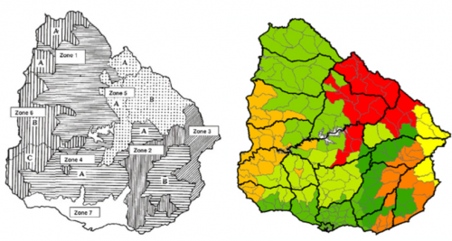
Based on national research on agro-ecological zones, the country was divided into 7 zones, defined by soil types, the type and quality of the pastures, and the dominant production systems. The cattle population was divided into 9 sub-categories: bulls, breeding cows, wintering cows, bulls >3 years old, steers 2-3 years, bulls 1-2 years, heifers >2 years, heifers 1-2 years old, and calves. Within each of the 7 zones, data on the livestock population was obtained at the administrative level of Police Sections, an administrative division, on average 7000 hectares in size, that is the spatial basis for collection of agricultural statistics. Information on the production and feeding systems, and animal performance was obtained for each of the 7 zones from national publications or expert judgement from the group of experts.

Figure 1: Division of Uruguay’s national territory by agro-ecological zone (left panel) and by combination of agroecological zone and administrative regions (right panel)

Source: Uruguay BUR1


Resources

Uruguay BUR 1.

GRA and CCAFS (n.d.) Livestock development and climate change: the benefits of advanced greenhouse gas inventories.


Author: Andreas Wilkes, Values for development Ltd (2019)